Twist: Control Infrastructure
kinematic and dynamic infrastructure to build high-level robot behaviors
Commanding high-level behaviors on Twist requires both low-level firmware (refer to the Kod*Lab Mjbots SDK project page) and mid-level control infrastructure. I discuss the latter on this page. This project is under the supervision of J. Diego Caporale.
Overview
The Twist software is built within the Kod*Lab Mjbots SDK ecosystem. The control infrastructure for Twist consists of kinematic and dynamic robot descriptions, handling of robot-specific inputs, and logging. Sensing (i.e., IMU, motor torques) also falls under this label, but is handled through the underlying SDK.
I co-developed forward, inverse, and single rigid body (SRB) kinematic and dynamic models for working with Twist, and implemented them into modular classes and implementations using the SDK framework. Specifically, I authored the following classes to implement these functionalities.
| Class (Template) | Description |
|---|---|
TwistBehaviorLoop | An implementation of MjbotsBehaviorLoop defining the control loop parameters, active robot behaviors, and input/logging quantities for Twist. |
TwistRobot | An implementation of RobotBase storing information about the robot joints, limbs, kinematics, dynamics, and sensors. |
TwistLimb | A class providing computations for forward and inverse limb kinematics. |
TwistKinematic | A class providing computations for forward and inverse robot kinematics. |
SingleRigidTorso | A class providing computations relating to the single rigid body model of the robot. |
MjbotsBehaviorLoop and RobotBase are Kod*Lab Mjbots SDK classes. The robot kinematic and dynamic models are discussed at length in the remainder of this page.
Robot Anatomy
Twist is a 13-actuated-degree-of-freedom quadruped, with three actuated joints per limb and a single actuated joint in the spine. The limb joints control adduction/abduction (\(\theta_{A_i}\)), hip pitch (\(\theta_{H_i}\)), and knee pitch (\(\theta_{K_i}\)). Limbs are identified by index \(i \in [0, 3]\) as defined in the table below. The spine joint angle is indicated by \(\alpha\).
| \(i\) | Limb |
|---|---|
| 0 | Front-Left |
| 1 | Rear-Left |
| 2 | Front-Right |
| 3 | Rear-Right |

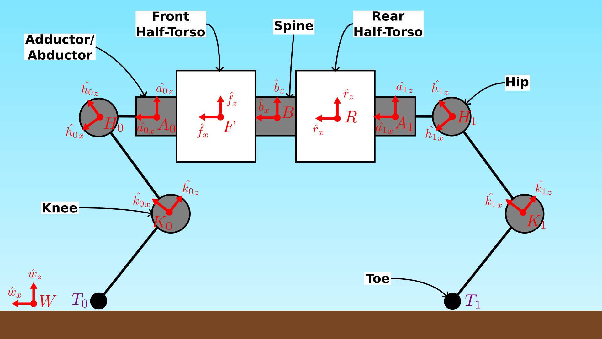
A diagram of the robot bodies and reference frames is provided above. These reference frames are defined as follows.
| Frame | Description |
|---|---|
| \(B\) | A virtual body frame made by averaging the \(F\) and \(R\) frames. |
| \(F\) | Frame fixed in the front half-torso. Shares an origin with \(B\). |
| \(R\) | Frame fixed in the rear half-torso. Shares an origin with \(B\). |
| \(A_i\) | Frame fixed in the adduction/abduction actuator for limb \(i\). |
| \(H_i\) | Frame fixed in the hip actuator for limb \(i\). |
| \(K_i\) | Frame fixed in the knee actuator for limb \(i\). |
Taking \(B\) as the trunk, these frames form a branching tree reaching the most extant knee frames \(K_i\) via a series of simple rotations (which are functions of the joint angles) and fixed translations defined as follows.
| Rotation | Axis | Angle |
|---|---|---|
| \({}^{B} R_{F}\) | \(+\hat{x}\) | \(\frac{\alpha}{2}\) |
| \({}^{B} R_{R}\) | \(+\hat{x}\) | \(-\frac{\alpha}{2}\) |
| \({}^{S} R_{A_i}\) | \(+\hat{x}\) | \(\theta_{A_i}\) |
| \({}^{A_i} R_{H_i}\) | \(+\hat{y}\) | \(\theta_{H_i}\) |
| \({}^{H_i} R_{K_i}\) | \(+\hat{y}\) | \(\theta_{K_i}\) |
For example, the rotation from the front-left knee frame to the virtual body frame can be decomposed into a series of simple rotations as follows:
\[{}^B R_{K_0} = {}^B R_{F} {}^F R_{A_0} {}^{A_0} R_{H_0} {}^{H_0} R_{K_0}.\]Forward Kinematics
The forward kinematics describe the body-frame toe positions via joint angles.

Limb Kinematics
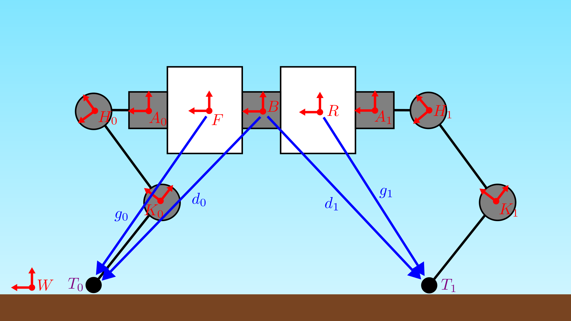
First, we compute the limb forward kinematics (i.e., a single toe position in the corresponding front or rear half-torso frame). Let \(g_i\) be the vector from a half-torso origin to a corresponding toe,
\[g_i = r^{T_i / S} = r^{T_i / K_i} + r^{K_i / H_i} + r^{H_i / A_i} + r^{A_i / S},\]where the frame \(S\) is given by \(S = \begin{cases} F ,& i \in \{0, 2\} \\ R ,& i \in \{1, 3\} \end{cases}\). The toe forward kinematics for a limb \(i\) are given by
\[{}^S g_i = {}^S r^{A_i / S} + {}^S R_{A_i} \left( {}^{A_i} r^{H_i / A_i} + {}^{A_i} R_{H_i} \left( {}^{H_i} r^{K_i / H_i} + {}^{H_i} R_{K_i} {}^{K_i} r^{T_i / K_i} \right) \right).\]Partially differentiating in the body frame with respect to the joint angles yields the forward limb Jacobian from the half-torso:
\[J_i = {}^{S} D g_i = \begin{bmatrix} {}^S R_{A_i} \hat{s}_x \times \left( {}^{A_i} r^{H_i / A_i} + {}^{A_i} R_{H_i} \left( {}^{H_i} r^{K_i / H_i} + {}^{H_i} R_{K_i} {}^{K_i} r^{T_i / K_i} \right) \right) \\ {}^S R_{A_i} {}^{A_i} R_{H_i} \hat{s}_y \times \left( {}^{H_i} r^{K_i / H_i} + {}^{H_i} R_{K_i} {}^{K_i} r^{T_i / K_i} \right) \\ {}^S R_{A_i} {}^{A_i} R_{H_i} {}^{H_i} R_{K_i} \hat{s}_y \times {}^{K_i} r^{T_i / K_i} \end{bmatrix}^{\intercal},\]which can be used to move between half-torso- and joint-space velocities. As \(J_i\) is a square, \(3 \times 3\) matrix, we are fully actuates for toe positioning in the half-torso frames.
Robot Kinematics
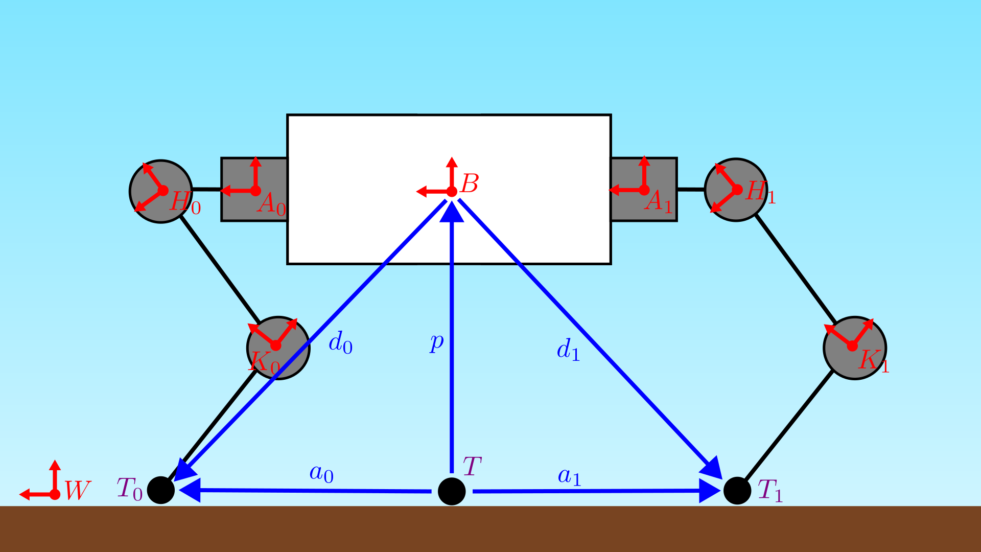
Now, we use the limb kinematics to build the full-body kinematics. Let \(d_i\) be the vector from the virtual body origin to a given toe,
\[d_i = r^{T_i / B}.\]In terms of the limb kinematics, this can be written for any given toe as
\[{}^B d_i = {}^B r^{S / B} + {}^B R_S {}^S g_i.\]Partially differentiating the full toe position vector above yields the spine-inclusive limb Jacobian,
\[J_i^{\mathrm{SI}} = {}^S D d_i = \begin{bmatrix} {}^B R_S J_i & \pm \frac{1}{2} {}^B R_S \hat{b}_x \times J_i \end{bmatrix}.\]Note that this non-square, \(3 \times 4\) matrix includes an additional column compared to the \(J_i\) due to the added spinal joint. This indicates that we are over-actuated for single-toe positioning in the body frame. Alternately, this can be expressed as a body Jacobian encompassing all four toes:
\[J = \begin{bmatrix} {}^B R_F J_0 & 0 & 0 & 0 & \frac{1}{2} {}^B R_F \hat{f}_x \times J_0 \\ 0 & {}^B R_R J_1 & 0 & 0 & -\frac{1}{2} {}^B R_R \hat{r}_x \times J_1 \\ 0 & 0 & {}^B R_F J_2 & 0 & \frac{1}{2} {}^B R_F \hat{f}_x \times J_2 \\ 0 & 0 & 0 & {}^B R_R J_3 & -\frac{1}{2} {}^B R_R \hat{r}_x \times J_3 \end{bmatrix}.\]Note that \(J\) is a \({12 \times 13}\) matrix, indicating that the robot is over-actuated for body-space toe positioning (which has 12 spatial DOF).
Body-Space and Joint-Space
The relationship between Cartesian body velocities and joint velocities is given by
\[\begin{bmatrix} \dot{x}_0 \\ \dot{x}_1 \\ \dot{x}_2 \\ \dot{x}_3 \end{bmatrix} = J \begin{bmatrix} \dot{\Theta}_0 \\ \dot{\Theta}_1 \\ \dot{\Theta}_2 \\ \dot{\Theta}_3 \\ \alpha \end{bmatrix},\]where \(\Theta_i = \begin{bmatrix} \theta_{A_i} & \theta_{H_i} & \theta_{K_i} \end{bmatrix}^{\intercal}\). Similarly, force vectors at the toes can be transformed to joint-space torques per
\[\tau = J^\intercal \begin{bmatrix} f_0 \\ f_1 \\ f_2 \\ f_3 \end{bmatrix}.\]Inverse Kinematics
The inverse kinematics describe the joint configuration or configurations which produce a desired toe position. As discussed previously, when the spine is used, the limbs are over-actuated for positioning tasks. To remedy this and avoid conflicting spine commands when computing inverse kinematics for multiple toes at once, we can simply pass the current spinal joint angle forward as a computation parameter, and compute inverse kinematics in the fully-actuated half-torso space.
More details on this computation will be provided soon!
Single Rigid Body Dynamics
For many behaviors, it is useful to describe the robot solely in terms of contact forces at the toes and the wrenches (forces and torques) they produce on the torso, ignoring limb dynamics. This is commonly referred to as a single rigid body (SRB) dynamics model as the limb dynamics are abstracted away. One of the benefits of using this approach is that it is easily adapted for different contact scenarios (e.g., cases where not all of the toes are in contact with the ground). For a rigid-torso quadruped (akin to Twist with a rigid spine), this is derived as follows.

More details on this model will be provided soon!